
In 2016, I created a project called Ex/Noise/CERN, experimental noise music inside CERN.

Satomi Matsuzaki of Deerhoof, in Ex/Noise/CERN Episode 1, 2015.
The crux of the project is juxtapositional: We take a boundary-stretching musician, immerse them in the world of the most cutting edge particle physics research in human history, operating at the extremes of knowledge, and then inspire them to do some manner of musical improvisation in one of the key, equally boundary-stretching (and visually arresting) experimental locations here at CERN, and make of film of it. This is admittedly high-concept, site-specific, experimental, improvisational performance, where the improv can take a lot of different possible forms.
The resulting film of the first episode, with Deerhoof, garnered some attention in the music and tech/sci press, and within four days of its release was among the top ten most watched videos that CERN has ever produced.
Because of its success, I often get asked two things about it:
1) When is the second episode coming out? A: Long story, but sometime.
2) Hey, you must do Large Hadron Collider (LHC) data sonification, too, yes?
My answer to this second question was always, No. The first episode of Ex/Noise/CERN and the sonification (making music or tones out) of LHC data are obviously two completely different things with very different intentions. But people kept asking about it, sometimes in the context of proposals for other Ex/Noise/CERN episodes where what’s produced musically may have some connection to collision data itself. It’s definitely an intriguing potential direction in which to go, but it’s somewhat orthogonal to my own original interests with ExNC.
To be able to answer the question as to why they’re very different from a more experienced perspective, I set out to research the concept of data sonification in more detail, to hopefully have something to show people when they asked about it.
Thus, sometime in 2016, I spent a few hours and made Gray: An Exercise in Large Hadron Collider Data Sonification, described here below.
Noise at CERN
Large Hadron Collider collisions don’t actually sound like much of anything.

Not loud.

Not loud, though perhaps echo-y.

Not loud, though there are some droning, industrial hums inside the ATLAS cavern.

Not loud. It’s an image.
So the proton collisions themselves don’t sound like much of anything at all, but they do produce an overwhelmingly large amount of very complex data.
Thus, when anyone talks about “sonifying” data — LHC data, satellite telescope data, genome sequencing data — they’re really talking about defining a mapping between data properties and tones audible to humans.
There are a large number of ways to do this, and some of the existing examples can get very inventive and wildly appeal to the physicist/coder/pop-scientist inside all of us.


Again, these are all impressive and evince a lot of time and effort to use our LHC collision data, as described at the above page, to create, “a result that while beautiful, is both musically and scientifically meaningful.” But all of these endeavors are fundamentally different from the intentions of Ex/Noise/CERN.
I kept getting asked about sonfication of LHC data in conjunction with Ex/Noise/CERN, however, and after many iterations of telling people, “This is something very different, and please check out all of these existing sonification projects by these other great people for the music-as-pedagogical-tool approach, which is not what Ex/Noise/CERN is”, I eventually posed myself a challenge exercise: What’s the simplest possible way to sonify LHC data?
Exercise: A simple approach to LHC data sonification —> Gray
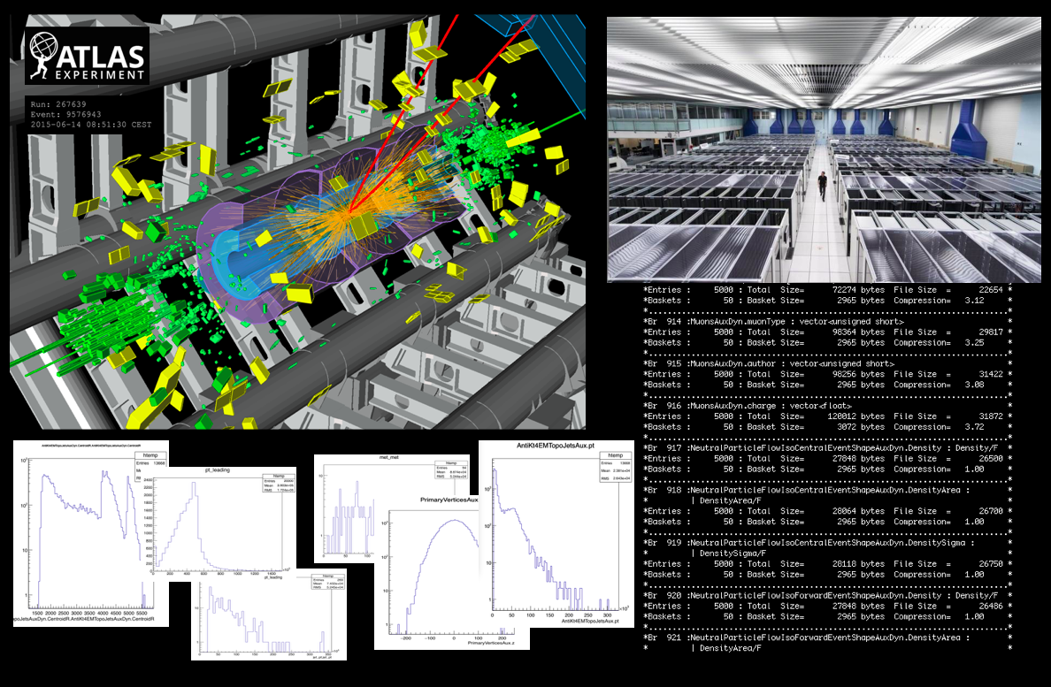
I started researching this question in the evening after a long day of coding and physics analysis with ATLAS, my experiment here at CERN, and after about four hours over the next couple of days, I arrived at the following.
Recall that sonification of LHC data involves defining a mapping between collision data properties and audible tones. We collide protons at a nominal rate of 40 MHz, or forty million times per second, at the LHC. We collect and store a tiny fraction of these, but we’re still collecting a data record of trillions of events, when all is said and done. Each one of these collisions will have a certain value for a broad range of properties or variables that are of interest for us to search for evidence of new particles. For example, each collision will contain a certain number of particles called muons that fly out from the interaction point and leave a track as they do so. So one event we record may have four muons in it. Another may have two. Another may have seven. One individual event isn’t so interesting on its own, but when you take billions or trillions of these events and plot a histogram of the number of muons per event, you will see a nice distribution, some kind of graph with a shape. This will resemble the distribution of muons-per-event that nature is sampling from to give us each individual proton collision.
Overwhelmingly, however, nearly all of these collision events will not be produced from a revolutionary new particle. They’re almost all produced from physics processes that we know and love and understand very well. Crucially, what we’re looking for when we search for evidence of new particles is some of these distributions that look distinctly different when a new particle produces them versus when our collision noise — or background — produces them. These new particle processes are very rare (otherwise we would have discovered them already), so what we’re trying to do is identify potential signals above a vast sea of background noise. We do this by looking at (in rather complex ways) a large number of these distributions of trillions of events to see if some of them contain deviations from the shapes that we didn’t expect.
And muons-per-event is only one of thousands of distributions we’re interested in as physicists. Another would be the transverse momentum values of these muons. Another would be the angles at which these muons fly away from the proton-proton collision point. Another would be all of these same variables but for photons instead of muons.
Thus, one straightforward way of turning LHC data into audible tones is by choosing a few of the numerous distributions of collision data properties that we collect and taking their ranges and mapping them to the range of tones or notes that humans can hear.

The Large Penderecki Collider.
This mapping can be simple: If one event has, for example, two muons, then play a high A on a piano, and if it has three muons, play a high B on a piano. Or this mapping can be somewhat complex: If one event has a muon in it, take the momentum value of that muon and map that value over to a certain range of tones that have been filtered through a noise generator that sounds like a buzzsaw.
I took some of our ATLAS collision data and selected only events containing two high-energy photons, chosen from among the trillions collected. I chose six variables.
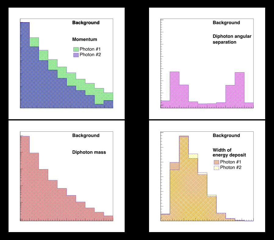
Each event will have some number for each of these six variables. The probability that an event will have some value of these variables is given by these distributions.
To mimic what we’re interested in as physicists, I chose variables where the distributions for background events are very different from signal events. In this example, events that contain only two photons can be the result of background processes or could be the result of a particle called a hyper-dimensional graviton that may live in extra dimensions of space beyond the three you and I experience, and could help explain why gravity is so insanely weak compared to all of the other forces of nature.
A graviton signal should look very different from a diphoton background distribution. I chose some distributions where this would be the case.
Note that we haven’t yet discovered a graviton, so we don’t really know what its properties are. Thus, we don’t have actual collision data with gravitons in it. To get a better sense as to how new particles like gravitons might show up in our collision data, we use some well-understood theoretical models and produce simulated events that, in the final data format, are equivalent to our collision data. But they’re not collision data. They’re simulations. Here, I’m using both collision data and, for the graviton signal, simulated events.

This is nearly the simplest thing one could do.
I took a similarly simple approach toward turning these into sounds that resembled music.
Each event is unique, so each event should sound unique. The raw numbers that compose these distributions themselves aren’t that interesting, but the shapes are, as discussed.
So I took the shapes and mapped their ranges into audible sounds such that each event will have a completely unique and random sonic fingerprint, in a way that background and signal events will be aurally distinguishable.
Each event gets one second.
We store and analyze our LHC collision data in a data format called ROOT, which is written in C++, but for which people have written very good python wrappings/interfaces. Since it’s straightforward to interpret LHC collision data via python, I used pyo, a python/C-based digital signal processing project.
Much of my time was spent playing around with the various signal generators built into pyo. There are many of them, and they’re fun. I played around with mixing and matching the sounds and fiddling with the parameters inside, adjusting them to ranges that sounded interesting to me. Then I played around with different ways of combining some of the variables in each collision event so that the resulting sounds would map into these ranges and generators inside pyo that I’d chosen.

The fourth component needed to do the simplest thing possible was the beat. I wanted something deep and subtle, with the number of taps per second based on “pileup”, the average number of collisions per proton-bunch crossing in 2015. In the following examples, it’s 16.

To produce the initial pieces of music, then, I processed ten events of background and ten of signal.

They should sound different. They do.
This becomes clear when comparing these outputs to the input distributions.

Finally, to create some longer pieces of music, I threw in some simulated events containing top and anti-top quarks, for fun.

Thus, I arrived at some sixty-second pieces, each of which represents sixty collision events, some real data, some simulated events, some of which contain diphoton background processes, some of which contain simulated graviton events, and some of which contain simulated top / anti-top quark events.
Then I produced a few with varying levels of pileup mapped to additional, overlapping beats.
In 2016 I had been invited to speak at Klangfestival, in Gallneukirchen, Austria, about particle physics, dark matter, the Higgs boson, and my research exploring the edges of knowledge here at CERN. The organizers were also aware of — and fans of — Ex/Noise/CERN. When I arrived for the festival, we were chatting about physics and music and improvisational noise. One thing led to another and they asked me if I played music myself. I used to play woodwinds — and had a jazz combo in high school, with me on alto — but I don’t play saxophone anymore. I mentioned that I had recently done this Gray: An Exercise in LHC Data Sonification thing, just as a few-hours proof-of-concept exercise for myself, and they said, “Whoa, we have an impromptu noise improv band playing tonight before your talk! You should perform with them!” And I said, “Nah.” And they said, “Yeah!” And I said, “Okay.”

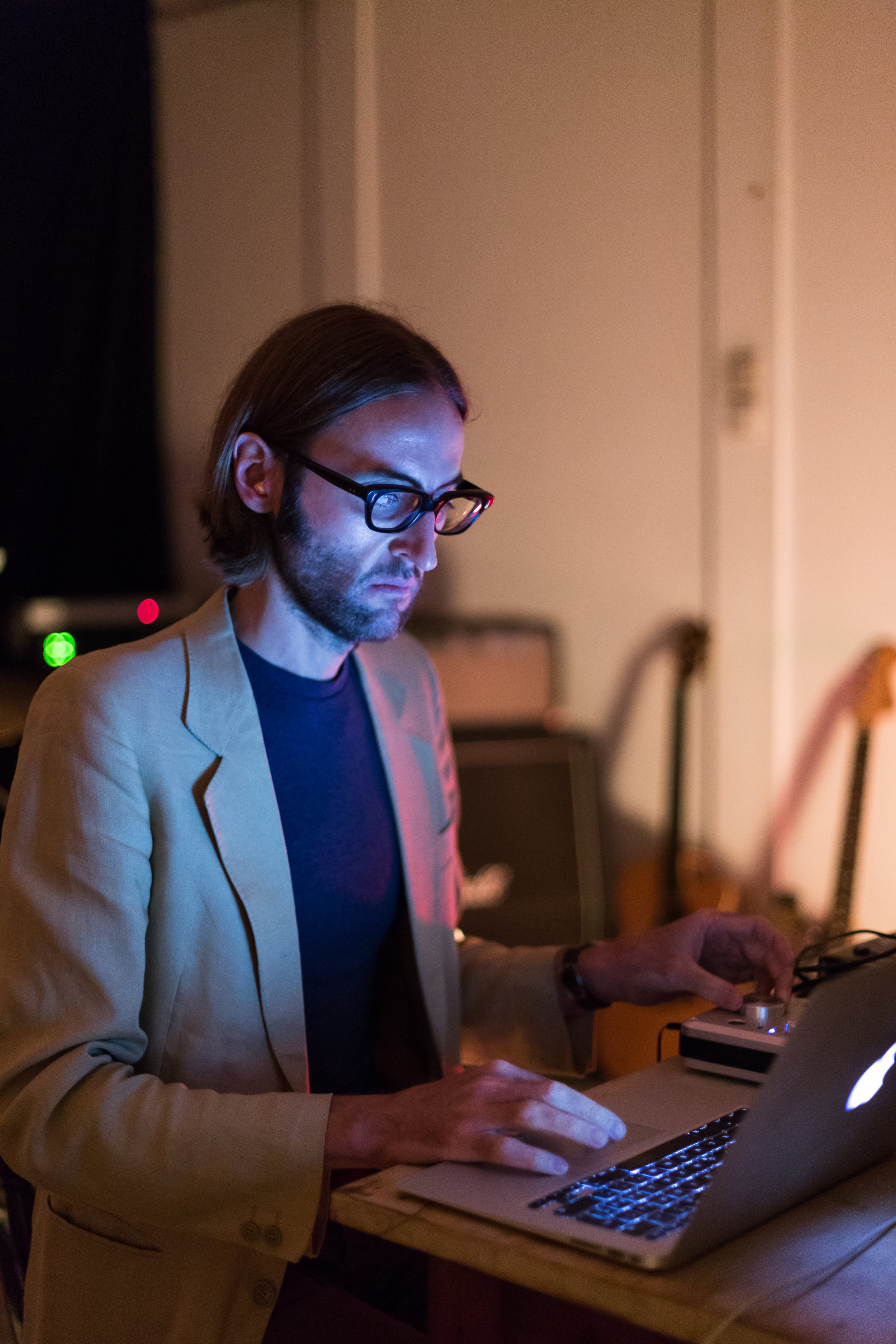
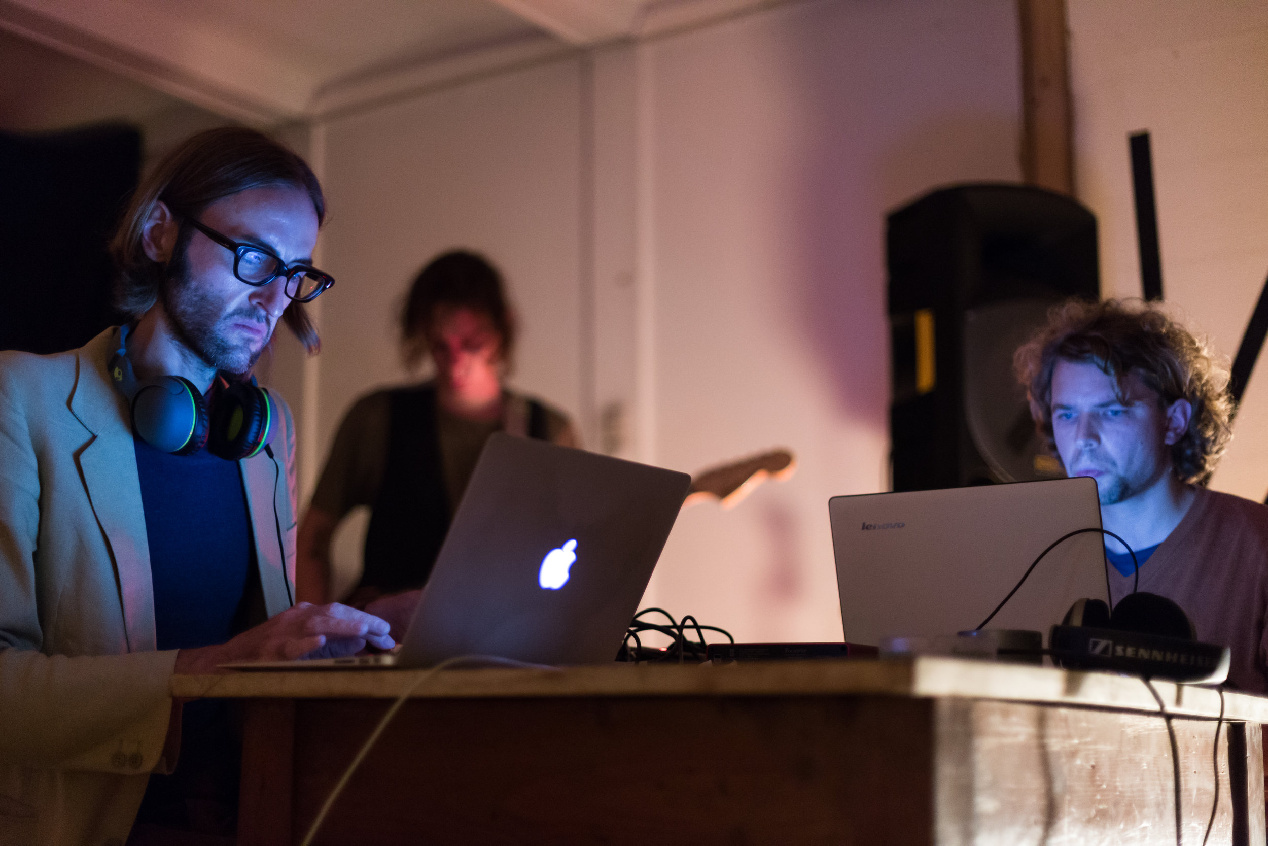
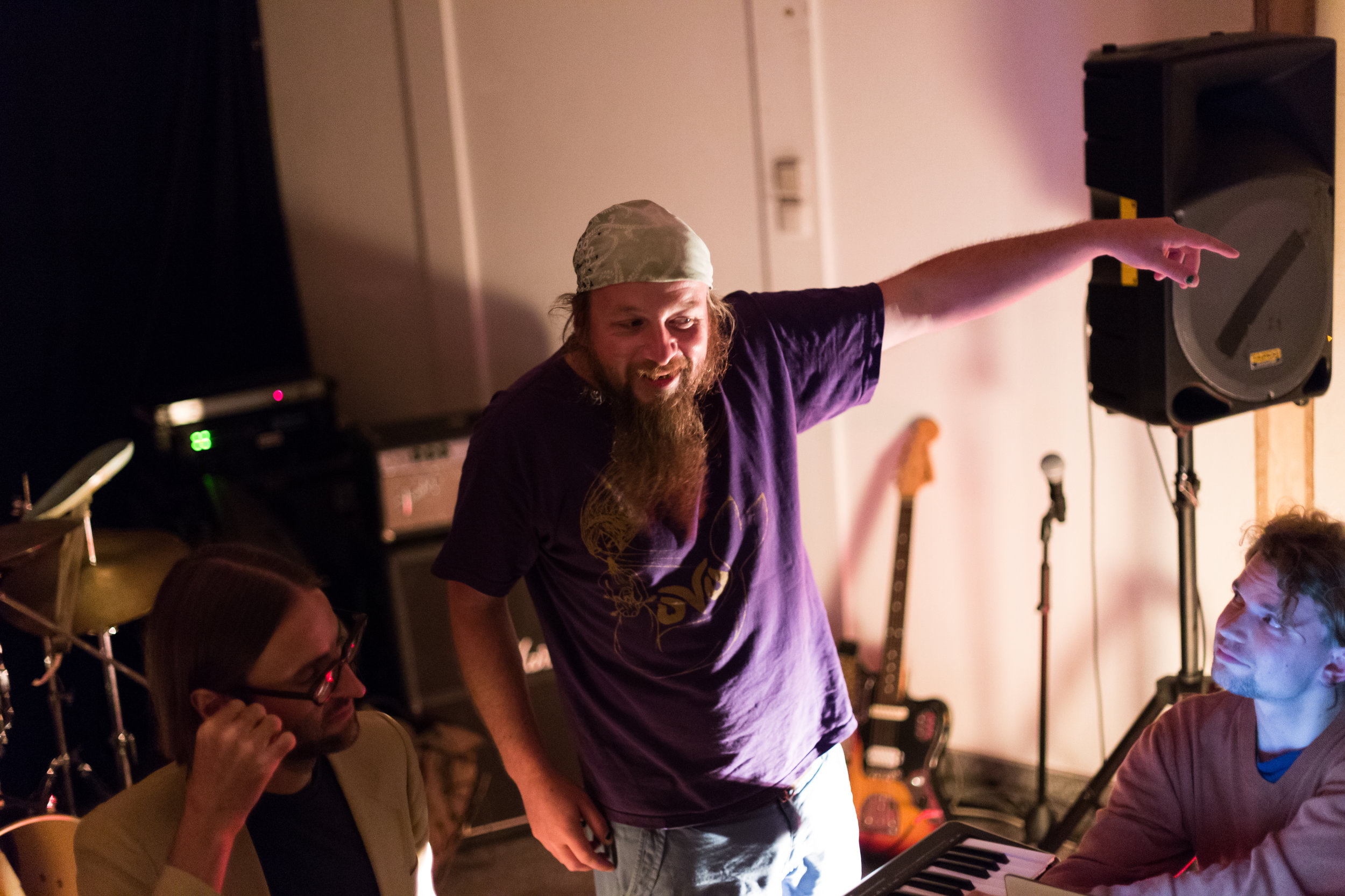
My performance, in this case, was me adjusting parameters in my code and then producing thirty- or sixty-second files that I would play. I couldn’t adjust the tempo at the time, so the band was essentially reacting to what I would play and then, depending upon their reactions, I would produce a new file with parameter adjustments to match or morph and play that.
It worked well with a live noise band. We recorded our first album, which went to number one in two hundred countries, and that spring we sold out Madison Square Garden for six straight nights.
Gray: An Exercise in Large Hadron Collider Data Sonification is named for Eileen Gray.